🧔 - me
👩🔬 - volunteer, please
why?
🧔 - Let's look at some data.
data
🧔 - Wow, that's a lot of data.
🧔 - Let's see if we can figure anything out with this data.
🧔 - How many data sets are there?
len(data['dataset'].unique())
And they are...
data['dataset'].unique()
🧔 - Wow, that's a lot of data sets.
🧔 - Let's calculate the mean values for the x values.
data.groupby('dataset')["x"].mean()
🧔 - Hmmm... 🤔
🧔 - They are all roughly the same!
🧔 - Let's calculate the mean values for the y values.
data.groupby('dataset')["y"].mean()
🧔 - Hmmm... 🤔
🧔 - They are all roughly the same!
🧔 - Let's calculate the mean and sd values for both the x and y values.
d = {}
d['mean x'] = data.groupby('dataset')["x"].mean().tolist()
d['mean y'] = data.groupby('dataset')["y"].mean().tolist()
d['sd x'] = data.groupby('dataset')["x"].std().tolist()
d['sd y'] = data.groupby('dataset')["y"].std().tolist()
df = pd.DataFrame(data=d)
df.index.name = "data sets"
df
🧔 - 😲 They are all roughly the same! 😲
🧔 - In conclusion, these data sets must all be the same!
🧔 - ✨ Thanks for coming to my TED talk! ✨
🧔 - Have a great day! 😃
👩🔬 - Wait..
🧔 - yes?
👩🔬 - have you looked at the data?
🧔 - why?
👩🔬 - sometimes statistics don't tell the whole story. Convert the data into another format and see if these trends continue.
🧔 - fine...
👩🔬 - Let's try sound, this is call 💥sonification💥
sr = 22050
T = .1
t = np.linspace(0, T, int(T*sr), endpoint=False)
x = data[data['dataset'] == "A"]["x"].multiply(10).sample(n=100, random_state=1).tolist()
e = []
for a in x:
    e.append(0.5*np.sin(2*np.pi*a*t))
sound1 = np.array(e)
ipd.Audio(sound1.flatten(), rate=sr)
sr = 22050
T = .1
t = np.linspace(0, T, int(T*sr), endpoint=False)
x = data[data['dataset'] == "B"]["x"].multiply(10).sample(n=100, random_state=1).tolist()
e = []
for a in x:
    e.append(0.5*np.sin(2*np.pi*a*t))
sound2 = np.array(e)
ipd.Audio(sound2.flatten(), rate=sr)
🧔 - WOW! This sound is banging. I am going to sample this for my rave band.
👩🔬 - you're not in a band
😎 - yes I am
👩🔬 - ...
🧔 - ...
🧔 - WOW! You can hear a difference! I wish I could see the sound!
👩🔬 - You can! Remember, visualizations are just representations of signals. See...
fig

fig

🧔 - oww, that's pretty...
👩🔬 - This is one of the big "gotchas" of data visualizations. It is part data and part art.
🧔 - why is this a "gotcha"?
👩🔬 - because art is subjective. It is a bit of a balancing act between "What looks cool!" and "What looks precise."
🧔 - so how do I build one of these visualatrons?
👩🔬 - visualizations. Well, there are two factors to consider when building visualatrons, I mean visualization. They are the spatial or planar encoding and the visual or retinal encoding. For now, we will call them spatial and visual encodings. Let's start with the visual encodings.
🧔 - ohhh
🧔 - ahhh
🧔 - whhhat?
👩🔬 - When you translate signals to symbols, we call these symbols glyphs and the process of connecting glyphs with data, 💥semiotics💥
🧔 - Can you encode multiple things with objects?
👩🔬 - Yep, but we need to ask, are the data integral or separable? Let's look at an example.
👩🔬 - Let's map our x and y values two different ways and see if we can pick how best to map our values.
🧔 - I think I am starting to get it. I have an idea! Let's check out all the datasets based on these visual encodings.
🧔 - There is definitely something going on with these datasets. But I am still not convinced that some are the same.
👩🔬 - Good call, maybe we should discuss the last component of visualizations...
🧔 - tacos?
👩🔬 - I thought we were finally having a breakthrough. No, the spatial component. This is the most important component of them all. It's like the old saying...
🧔 - you are what you eat?
👩🔬 - You're hungry, aren't you.
🧔 - yes.
👩🔬 - Well, the saying is... location, location, location.
👩🔬 - The spatial component is all about using space to code data. Let's take a look at two plots.
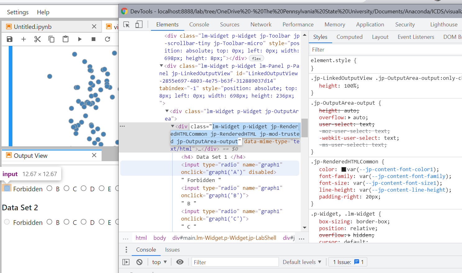
🧔 - wait, what's that forbidden one?
👩🔬 - what forbidden one?
🧔 - the one that says "forbidden!""
👩🔬 - oh, we can't touch that one.
🧔 - hmmm... let's see if I can fix this.